RBSE Class 12 Maths Notes Chapter 6 Application of Derivatives

These comprehensive RBSE Class 12 Maths Notes Chapter 6 Application of Derivatives will give a brief overview of all the concepts.

RBSE Class 12 Maths Chapter 6 Notes Application of Derivatives

Introduction:
In previous chapter, we have learnt how to find derivative of composite functions, inverse trigonometric functions, implicit functions, exponential functions and logarithm functions. In this chapter, we will study applications of the derivative in various disciplines.

Rate of Change of Quantities:
Let y = f(x) be a function of x.
Let Δy be the change in y corresponding to a small change Δx in x.
Then, \(\frac{\Delta y}{\Delta x}\) represents the change in y due to a unit change in x. In other words, \(\frac{\Delta y}{\Delta x}\) represents the average rate of change of y with respect to x as x changes from x to x + Δx.
As x → 0, the limiting value of this average rate of change of y with respect to x in the interval [x, x + Δx] belongs the instantaneous rate of change of y with respect to x.

Thus,
\(\lim _{\Delta x \rightarrow 0} \frac{\Delta y}{\Delta x}\) = Instantaneous rate of change of y w.r.t. x
⇒ \(\frac{d y}{d x}\) = rate of change of y w.r.t x [\(\lim _{\Delta x \rightarrow 0} \frac{\Delta y}{\Delta x}=\frac{d y}{d x}\)]
The word 'instantaneous' is of the dropped. dy
Hence, \(\frac{d y}{d x}\) represents the rate of change of y with respect to x for a definite value of x.

Note:
The value of \(\left(\frac{d y}{d x}\right)\)x = x₀ represents the rate of change of y w.r.t x at x = x₀

 

Rate of Change of Two Variables
If two variables x and y are varying w.r.t. another variable t, i.e., if
x = f(t) and y = g(t), then by chain rule
\(\frac{d y}{d x}=\frac{d y}{d t} / \frac{d x}{d t}\), where \(\frac{d x}{d t}\) ≠ 0
Thus, the rate of change of y w.r.t. x can be calculated using the rate of change of y and that of x both w.r.t. t.

Note:
\(\frac{d y}{d x}\) is positive, if y increases as x increases and it is negative, if y decreases as x increases.

Marginal Cost and Marginal Revenue
Marginal Cost
Marginal cost represents the instantaneous rate of change of the total cost at any level of output.
If C(x) represents the cost function for x units produced, then marginal cost (MC) is given by MC = \(\frac{d}{d x}\)(C(x)

Marginal Revenue
Marginal revenue represents the rate of change of total revenue with respect to the number of items sold at an instant.
If R(x) is the revenue function for x units sold, then marginal revenue (MR) is given by
MR = \(\frac{d}{d x}\) R(x)

Increasing And Decreasing Functions:
In this section, we will use differentiation to find out whether a function is increasing or decreasing or none.

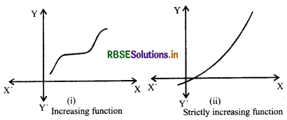
Increasing function:
Function f(x) is called increasing function in open interval (a, b) if
x₁ < x₂ ⇒ f(x₁) ≤ f(x₂), ∀ x₁ x₂ ∈ (a, b)

Strictly increasing function :
Function f(x) is called strictly increasing function in open interval (a, b) if
x₁ < x₂ ⇒ f(x₁) < f(x₂), ∀ x₁ x₂ ∈ (a, b)

Decreasing function:
Function f(x) is called decreasing function in open interval (a, b) if
x₁ < x₂ ⇒ f(x₁) ≥ f(x₂), ∀ x₁ x₂ ∈ (a, b)

Strictly decreasing function :
Function f(x) is called strictly decreasing function in open interval (a, b) if
x₁ < x₂ ⇒ f(x₁) > f(x₂), ∀ x₁ x₂ ∈ (a, b)

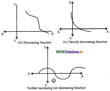
For a given interval I ⊆ R, function f increases for some values in I and decreases for other values in I, then we say function is neither increasing nor decreasing.
If there exists an open interval I containg x0 such that
x₁ < x₂ in I ⇒ f(x₁) > f(x₂)
Similarly, the other cases can be clarified.

Note:
A function f is said to be increasing at x if there exists an interval I = (x₀ - h, x₀ + h), h > 0 such that for x₁ x₂ ∈ I.

Theorem 1.
Let f be continuous on [a, b] and differentiable on the open interval (a, b). Then
(a) f is increasing in [a, b] if f' (x) > 0 for each x ∈ (a, b).
(b) f is decreasing in [a, b] if f' (x) < 0 for each x ∈ (a, b).
(c) f is a constant function [a, b] if f' (x) = 0 for each x ∈ (a, b).
Proof:
(a) Let x₁ x₂ ∈ [a, b] be such that x₁ < x₂.
Then, by mean value theorem, there exists a point c between x₁ and x₂, such that.
f(x₂) - f(x₁) = f(c)(x₂ - x₁)
i.e. f(x₂) - f(x₁) > 0 (as f (c) > 0 (given))
i.e. f(x₂) > f(x₁)
Thus, we have
x₁ < x₂ => f(x₁) < f(x₂), for all x₁ x₂ ∈[a, b]
Hence, f is an increasing function in [a, b].
The proofs of part (b) and (c) are similar.

Remarks:

• f is strictly increasing in (a, b) if f' (x) > 0 for each x ∈ (a, b).
• f is strictly decreasing in (a, b) if f' (x) < 0 for each x ∈ (a, b).
• A function will be increasing (decreasing) in R if it is increasing (decreasing) in every interval of R.

Tangents And Normals:
In this section we shall use differentiation to find the equation of the tangent line and the normal line to a curve at a given point.
A line which touches the curve at a single point is called tangent at a point and if a line is perpendicular to the tangent at the point of contact, then it is called normal.

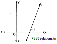
Slope of a line: The trigonometrical tangent of the angle that a line makes with the positive direction of X-axis in anti-clockwise direction is called the slope or gradient of the line. The slope of line is generally denoted by m.
Thus, slope of line m = tan θ

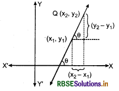
Slope of line by coordinates of two points:
Let P(x₁, y₁) and Q(x₂, y₂) are two points on a line, then slope of line (tan θ), m = \(\frac{y_{2}-y_{1}}{x_{2}-x_{1}}\)

Slope of line by equation of line:
Let equation of line be ax + by + c = 0, then slope of line is m such that:
m = \(\frac{-a}{b}=-\frac{\text { coefficient of } x}{\text { coefficient of } y}\)
Note that the slope of the tangent to the curve y = f(x) the point (x₀, y₀) is given by \(\left.\frac{d y}{d x}\right]_{\left(x_{0}, y_{0}\right)}\) = f'(x₀)). So the equation of the tangent at (x₀, y₀) to the curve y = f (x) is given by

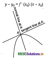
Also, since the normal is perpendicular to the tangent, the slope of the normal to the curve y = f (x) at (x₀, y₀) is \(\frac{-1}{f^{\prime}\left(x_{0}\right)}\) if f' (x₀) ≠ 0. Therefore, the equation of the normal to the curve y = f(x) at (x₀, y₀) is given by
y - y₀ = \(\frac{-1}{f^{\prime}\left(x_{0}\right)}\)(x -x₀)
i.e (y - y₀)f' (x₀) + (x - x₀) = 0

Note:
If a tangent line to the curve y = f(x) makes an angle θ with x-axis in the positive direction, then \(\frac{d y}{d x}\) = slope of the tangent = tan θ.

Particular cases

• If slope of the tangent line is zero, then tan θ = 0 and so θ = 0° which means the tangent line is parallel to the x-axis. In this case, the equation of the tangent at the point (x₀, y₀) is given by y = y₀.
• If, θ = \(\frac{\pi}{2}\) then tan θ = ∞, which means the tangent

line is perpendicular to the x-axis, i.e., parallel to the y-axis. In this case, the equation of the tangent at (x₀, y₀) is given by x = x₀.

Angle of Intersection of two Curves :
At the point-of intersection of two curves, angle formed between their corresponding tangents is called angle of intersection of two curves.
Let y = f(x) and y = g(x) are two equations of curves. Let two curves intersect at point P.
Let PT₁ and PT₂ are two tangents at curves which interesect each other at point P and Φ is angle between them if tangents makes angle Ψ₁ and Ψ₂ with the x-axis then

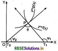
m₁ = tanΨ₁ = slope of curve y = f(x) at point P
and m₂ = tanΨ₂ = slope of curve y = g(x) at point P

From figure, it is clear that
Φ = Ψ₁ - Ψ₂
∴ tan Φ = tan (Ψ₁ - Ψ₂)
⇒ tan Φ = \(\frac{\tan \psi_{1}-\tan \psi_{2}}{1+\tan \psi_{1} \tan \psi_{2}}\)
⇒ tan Φ = \(\frac{\left(\frac{d y}{d x}\right)_{y=f(x)}-\left(\frac{d y}{d x}\right)_{y=g(x)}}{1+\left(\frac{d y}{d x}\right)_{y=f(x)} \times\left(\frac{d y}{d x}\right)_{y=g(x)}}\)
Another angle between tangents is 180° - Φ. Generally smaller angle is taken as angle between tangents.

Orthogonal Curves: If angle of intersection of two curves is right angle or intersecting curves are perpendicular at their intersection are said to be orthogonal.
When curves will be orthogonal then
Φ = \(\frac{\pi}{2}\)
In this case, m₁ m₂ = - 1
⇒ \(\left(\frac{d y}{d x}\right)\) y = f(x) = \(\left(\frac{d y}{d x}\right)_{y=g(x)}\) = -1

Errors And Approximations:
In this section, we will use differentials to approximate value of certain quantities.
Let f : D → R, D ⊂ R, be a given function and let y = f(x). Let Δx denotes a small increment in x. Recall that the increment in y corresponding to the increment in x, denoted by Δy, is given by Δy = f(x + Δx) - f(x). We define the following:

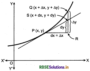
(i) The differential of x, denoted by dx, is defined by dx = Δx.
(ii) The differential of y, denoted by dy, is defined by
Thus, f(x + Δx) ≈ f(x) + f'(x). Δx
⇒ f(x + Δx) ≈ y + Δy [∴ Δy = dy]
In case dx = Δx is relatively small when compared with x, dy is a good approximation of Δy and we denote it by dy.

Note: In view of the above discussion and figure, we may note that the differential of the dependent variable is not equal to the increment of the variable where as the differential of indepedent variable is equal to the increment of the variable.

Some Important Errors

• Absolute error : Error in x, Δx is called absolute error.
• Relative error: If Δx is error in x then \(\frac{\Delta x}{x}\) is called relative error in x.
• Percentage error: If Δx is error in x then (\(\frac{\Delta x}{x}\) × 100) is called percentage error in x.

Maxima And Minima:
Definition : Let f be a function defined on an interval I. Then
(a) f is said to have a maximum value in I, if there exists a point c in I such that f(c) > f(x), for all x ∈ I
The number f(c) is called the maximum value of/in 1 and the point c is called a point of maximum value of f in I.
(b) f is said to have a minimum value in l, if there exists a point c in I such that f(c) < f(x), for all x ∈ I.
The number f(c), in this case, is called the minimum value of f in I and the point c, in this case, is called a -point of minimum x value of f in I.
(c) f is said to have an extreme value in I if there exists a point c in I such that f(c) is either a maximum value or a minimum value of f in I.
The number f(c), in this case, is called an extreme value of f in 1 and the point c is called an extreme point.

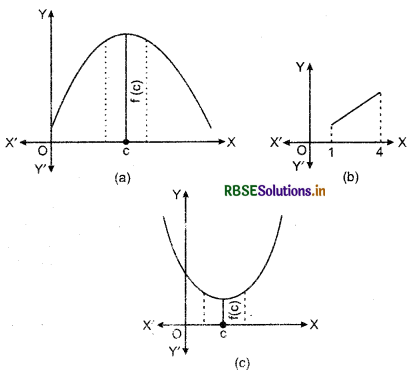
Remark : In figure (a), (b) and (c), we have exhibited that graphs of certain particular functions help us to find maximum value and minimum value at a point. In fact, through graphs, we can even find maximum f minimum value of a function at a point at which it is not even differentiable.

Example: Find the maximum and the minimum value, if any, of the function/given by
f(x) = x², x ∈ R
Sol. From the graph of the given function, we have f(x) = 0 if x = 0. Also
f(x) ≥ 0, for all x ∈ R

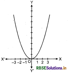
Therefore, the minimum value of f is 0 and the point of minimum value of f is x = 0. Further, it may be observed from the graph ot the function that f has no maximum value and hence no point of maximum value of f in R,
Note : If we restrict the domain of f to [- 2, 1], only then/will have maximum value (- 2)² = 4 at x = - 2.

Monotonic function: The function which is maximum or minimum at the end points of the defined domain is called monotonic function.
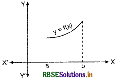
Monotonic increasing function : The function which is increasing in its defined domain, is called monotonic increasing function.

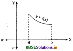
Monotonic decreasing function : The function which is deceasing in its defined domain is called monotonic decreasing function.

Note : By a monotonic function f in an interval I, we mean that f is either increasing in I or decreasing in I.

Nature of function (Increasing Decreasing) :
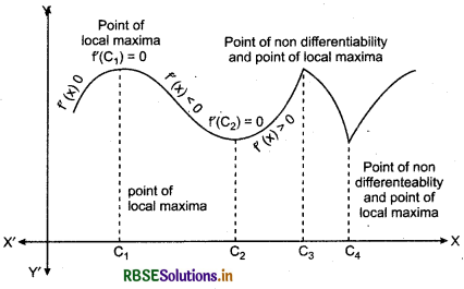
Let us now examine the graph of a function as shown in the following figure.

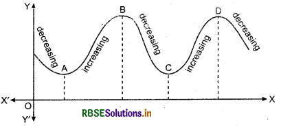
Observe that at points A, B, C and D on the graph, the function changes its nature from decreasing to increasing or vice-versa. These points may be called turning points of the given function. Roughly speaking, the function has minimum value in same neighbourhood (interval) of each of the points A and C which are at the bottom of their respective valleys. Similarly, the function has maximum value in same neighbourhood of points B and D which are at the top of their respetive hills. For this reason, the points A and C may be regarded as points of local minimum value (or relative maximum value) for the function.

The local maximum value and local minimum value of the function are referred to as local maxima and local minima, respectively, of the function.
We now formally give the following definition.

Definition 4.
Let f be a real value function and let c be an interior point in the domain of f. Then
(a) c is called a point of local maxima if there is an h > 0 such that f(c) > f(x), for all x in (c - h, c + h)
The value/(c) is called the local maximum value of f.

(b) c is called a point of local minima if there is an h> 0 such that f(c) < f(x), for all x in (c - h, c + h) The value f(c) is called the local minimum value of f. Geometrically, the above definition states that if x = c is a point of local maxima of f, then the graph of around c will be as shown in Fig. (a). Note that the function f is increasing, (i.e.,f(x) > 0) in the inverval (c - h, c) and decreasing (i.e.,f(x) < 0) in the interval (c, c + h).

This suggests that f(c) must be zero.

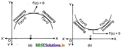
Similarly, if c is a point of local minima of f, then the graph of f around c will be as shown in figure (b). Here f is decreasing (i.e., f(x) < 0) in the interval (c - h, c) and increasing (i.e.,f(x) > 0) in the interval (c, c + h). This again suggest that f(c) to be zero.
The above discussion lead us to the following theorem (without proof).

Thereom 2.
Let f be a function define on an open interval I. Suppose c ∈ I be any point. If f has a local maxima or a local minima at x = c, then either f(c) = 0 or f is not differentiable at c.
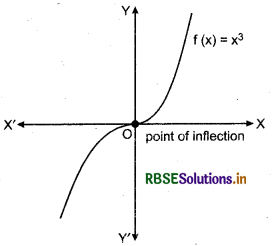
Remark : The converse of above theorem need not be true, that is, a point at which the derivative vanishes need not be a point of local maxima or local minima. For example, if f(x) = x³, then f(x) = 3x² and so f(0) = 0. But 0 is neither a point of local maxima nor a point of local minima.

Note: A point c in the domain of a function/at which either f(c) = 0 or f is not differentiable is called a critical point of f Note that if f is continuous at c and f(c) = 0, then there exists h > 0 such that f is differentiable in the inverval (c -h, c + h).
We shall now give a working rule for finding points of local maxima or points of local minima using only the first order derivatives.

Theorem 3.
(First Derivative Test): Let f be a function defined on an open interval I. Let/be continuous at a critical point c in I. Then

• If f(x) changes sign from positive to negative as x increase through c, i.e., if f(x) > 0 at every point sufficiently close to and to the left of c, and/(x) < 0 at every point suf-ficiently close to and to the right of c, then c is a point of local maxima.
• If f(x) changes sign from negative to positive as x increases through c, i.e., if f(x) < 0 at every point sufficiently close to and to the left of c, and f(x) > 0 at every point sufficiently close to and to the right of c, then c is a point of local minima.
• If f(x) does not change sign as x increase through c, then c is neither a point of local maxima nor a point of local minima. In fact, such a point is called point of inflection.

We shall now give another test to examine local maxima and local minima of a given function. This test is often easier to apply than the first derivative test.

Theorem 4.
(Second Derivative Test) : Let/be a function defined on an interval I and c ∈ I. Let f be twice differentiable at c. Then
(i) x = c is a point of local maxima if f(c) = 0 and f'(c) < 0 The value f(c) is local maximum value of f.
(ii) x = c is a point of local minima if f(c) = 0 and f'(c) > 0
In this case, f(c) is local minimum value of f.
(iii) The test fails if f(c) = 0 and f'(c) = 0
In this case, we go back to the first derivative test and find whether c is a point of local maxima, local minima or a point of inflection.

Note: As f is twice differentiable at c, we mean second order derivative of f exists at c.

Maximum and Minimum Values of a Function y in a Closed Inverval
Let us consider a function f given by
f(x) = x + 2, x ∈ (0,1)
Observe that the function is continuous on (0,1) and neither has a maximum value nor has a minimum value. Further, we may note that the function even has neither a local maximum value nor a local minimum value.

However, if we extend the domain of/to the closed interval [0,1], then f still may not have a local maximum (minimum) values but it certain by does have maximum value 3 = f( 1) and minimum value 2 = f(0). The maximum value 3 of f at x = 1 is called absolute maximum value (global maximum or greatest value) of f on the interval [0,1]. Similarly, the minimum value 2 of f at x = 0 is called the absolute minimum value (global minimum or least value) of f on [0,1].

Consider the,graph given in figure of a continuous function defined on a closed interval [a, d]. Observe that the function/has a local minima at x = b and local minimum value is f(b). The function also has a local maxima at x = c and local maximum value is f(c).

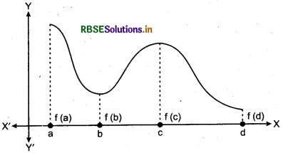
Also from the graph, it is evident that f has absolute maximum value f(a) and absolute minimum value f(d). Further note that the absolute maximum (minimum) value of f is different from local maximum (minimum) value of f.
We will now state two results (without proof) regarding absolute maximum and absolute minimum values of a function on a closed interval I.

Theorem 5.
Let f be a continuous funtion on an interval I = [a, b]. Then f has the absolute maximum value and f attains it at least once in I. Also, f has the absolute minimum value and attains it at least once in I.

Theorem 6.
Let f be a differentiable function on a closed interval I and let c be any interior point of I. Then
(i) f(c) = 0 if f attains its absolute maximum value at c.
(ii) f(c) = 0 if f attains its absolute minimum value at c.
In view of the above results, we have the following working rule for finding absolute maximum and f or absolute minimum values of a function in a given closed interval,[a, b].

Working Rule:
Step 1: Find all critical points of f in the interval, i.e., find points x where either f(x) = 0 or f is not differentiable.
Step 2. Take the end points of the inverval.
Step 3. At all these points (listed in step 1 and 2), calculate the values of f.
Step 4. Identify the maximum and minimum values of f out of the values calculated in step 3. This maximum value will be the absolute maximum (greatest) value of f and the minimum value will be the absolute minimum (least) value of f.

→ If a quantity y varies with another quantity x, satisfying some rule y = f(x), then \(\frac{d y}{d x}\) (or f(x)) represents the rate of change of y with respect to x and \(\left.\frac{d y}{d x}\right]_{x=x_{0}}\) (or f(x₀) represents the rate of change of y with respect to x at x = x₀.

→ If two variables x and y are varying with respect to another variable t, i.e., if x = f(t) and y = g(t), then by chain rule
\(\frac{d y}{d x}=\frac{d y}{d t} / \frac{d x}{d t}\), if \(\frac{d x}{d t} \) ≠ 0

→ A function f is said to be
(a) increasing on an interval (a, b) if x₁ < x₂ in (a, b) = f(x₁) < f(x₂) for all
x₁, x₂ ∈ (a, b).
Alternatively, if f(x) > 0 for each x in (a, b)

(b) decreasing on (a, b) If
x₁ < x₂in (a, b) ⇒ f(x₁) >f(x₂) for all x₁, x₂ ∈ (a, b) Alternatively, If/(x) < 0 for each x in (a, b)

→ The equation of the tangent at (x₀, y₀) to the curve y = f(x) is given by:
y - y₀ = \(\left.\frac{d y}{d x}\right]_{\left(x_{0}, y_{0}\right)}\) (x - x₀)

→ If \(\frac{d y}{d x}\) does not exist a t the point (x₀, y₀), then the tangent at this point is parallel to the y-axis and its equation is x = x₀.

→ If the tangent to a curve y = f(x) at x = x₀ is parallel to x = x₀

→ Equation of the normal to the curve y = f(x) at a point (x₀, y₀)is given by
y - y₀ = \(\frac{-1}{\left.\frac{d y}{d x}\right]_{\left(x_{0}, y 0\right)}}\)(x - x₀)

→ If \(\frac{d y}{d x}\) at the point (x₀, y₀) is zero, then equation of the normal is x = x₀.

→ If \(\frac{d y}{d x}\) at the point (x₀, y₀) does not exist, then the normal is parallel to x-axis and its equation is y = y₀.

→ Let y = f(x), Δx be a small increment in x and Δy be the increment iny corresponding to the increment in x, i.e., Δy = f(x + Δx) - f(x). Then dy is given by :
dy = f'(x) dx or dy = \(\left(\frac{d y}{d x}\right)\)Δx is a good approximation of Δy when dx = Δx is relatively small and we denote it by dy = Δy.

→ A point C in the domain of a function f at which either f'(c) = 0 or f is not differentiable is called a critical point of f.

→ First Derivative Test: Let f be a function defined on an open interval I. Let f be continuous at a critical point c in I. Then

• If f '(x) changes sign from positive to negative as x increases through c, i.e., if f'(x) > 0 at every point suficiently close to and to the left of c, and f'(x) < 0 at every point sufficiently close to and to the right of c, then c is a point of local maxima.
• If f'(x) changes sign from negative to positive as x increases through c, i.e., if f(x) < 0 at every point sufficiently close to and to the left of c, and f'(x) > 0
• at every point sufficiently close to and to the right of c, then c is a point of local maxima.
• If f'(x) does not change sign as x increases through c, then c is neither a point of local maxima nor a point of local minima. Infact, such a point is called point oj inflexction.

→ Second Derivative Test: Let f be a function defined on an interval I and cel. Let f be twice differentiable at c. Then.

• x = c is a point of local maxima if f'(c) = 0 and f'(c) < 0 The values f(c) is local maximum value of f
• x = c is a point of local minima if f'(c) = 0 and f(c) > 0. In this case, f(c) is local minimum value off.
• The test fails if f'(c) = 0 and f"(c) = 0
• In this case, we go back to the first derivative test and find whether c is a point of maxima, minima or a point of inflexion.