RBSE Class 12 Maths Notes Chapter 12 Linear Programming

These comprehensive RBSE Class 12 Maths Notes Chapter 12 Linear Programming will give a brief overview of all the concepts.

RBSE Class 12 Maths Chapter 12 Notes Linear Programming

Introduction:
We have studied solutions by graphical representation of linear inequations or equations. In many applications of mathematics, systems of inequations are included.
In this chapter, we shall apply the system of linear inequalities/equations to solve some real life problems.

Such type of problems which seek to maximize profit or minimize cost form a general class of problems called optimization problems. Thus, an optimization problem may involve finding maximum profit, minimum cost or minimum use of resources etc.

A special but a very important class of optimization problems is linear programming problem. The above stated optimization problem is an example of linear programming problem. Linear programming problems are of much interest because of their wide applicability in industry, commerce, management science etc. In this chapter, we shall study same linear programming problems and their solutions by graphical method.

Linear Programming Problem and its Mathematical Formulation:
A linear programming problem is one that is concerned with finding the optimal value (maximum or minimum value) of a linear function Z (called objective function) of several variables (say x and y), subject to the conditions that the variables are non-negative and satisfy a set of linear inequalities (called linear constraints).

 

Linear objective function :
Linear function Z = ax + by, where a, b are constants, which has to be maximized or minimized is called a linear objective function.

Constraints :
Constraints are the linear inequalities or equations or restrictions on the variables of a linear programming problem. In the constraints given in the general form of LPP there may be any one of the three signs ≤, =, ≥. For example, x > 0 or x < 0 or x > 7 or x + 2y ≤ 3.

Decision Variables:
Suppose Z = 250x + 75y is a linear objective function. Variables x and y are called decision variables.

Optimization Problem :
A problem which seeks to maximise or minimise a linear function (say of two variables x and y) subject to certain constraints as determined by a set of linear inequalities is called an optimization problem.

Mathematical Formulation of the Problem:
To formulate LPP, follow that following steps :

• Identify the objective function and express it as linear function of the given variables.
• Identify the set of constraints and express them as linear inequalities or equations.
• The set of all the variables satisfying the given constraints are obtained by mathematical method.
• We obtain the particular set of the variables which gives us the required objective function. For example - Minimum cost or maximum profit.

The process of the above formulation will be clear by the following example : 
Example :
A furniture dealer deals in only two items beds and sofasets. He has a space to store at most 50 pieces. He has ₹ 75,000 to invest. A bed costs ₹ 1,200 and a sofaset costs ₹ 1,500 and the profit on a bed is ₹ 125 while that on a sofaset is ₹ 200. Assuming that he can sell all the items that he made, formulate a linear programming problem. So as to maximize the profit.
Answer:
Let x and y be the required number of beds and sofasets.
∵ Number of beds and sofasets cannot be negative.
Hence, x ≥ 0, y ≥ 0 ...(1)
1,200x + 1,500y < 75,000
or
4x + 5y < 250 ...(2)
∵ The furniture dealer has a space to store 50 pieces, so total number of beds and sofasets should be equal to or less than 50.

Condition for the above is :
x + y < 50 ...(3)

Profit of ₹ 125 on each bed while ₹ 200 on each sofaset is shown by the following function :
Profit function P = 125x + 200y ... (4)
Hence, mathematical formulation is :
We have to maximize P = 125x + 200y
Subject to the constraints :
x ≥ 0, y ≥ 0, 4x + 5y ≤ 250; x + y ≤ 50

Graphical Method of Solving Linear Programming Problems:
Graphical method is the easiest method to solve any linear programming problem. This method is suitable for solving linear programming problem containing two decision variables only.

Comer Point Method :
This method is based on the fundamental extreme point theorem which is stated as: "An optimal solution of a linear programming problem (LPP), if it exists, occurs at one of the extreme (Comer) point of the convex polygon of the set of all feasible solution."
Following algorithm can be used to solve LPP in two variables graphically by using the comer point method :

• Step I. Formulate the given problem in the form of constraints and objective function.
• Step II. Convert all inequations into equations.
• Step III. Draw graph of all the equations and non-negative constraints. Now, we get same number of lines as the inequations and equations.
• Step IV. In this way, we obtain a feasible polygon bounded by these lines. The sides of the polygon satisfy all the constraints.
• Step V. Determine the coordinates of the vertices (comer points) or the feasible polygon.
• Step VI. We subsitute the coordinates of each vertex of the feasible polygon in objective function P and examine at which vertex the maximum profit or minimum cost is obtained. Here, we use the theorem which is fundamental in locating the point or points were optimum value is attained.

Example:
Solve the following linear programming problem graphically:
Minimum P = 2x - y subject to the constraints x + y ≤ 5, x + 2y ≤ 8 and x ≥ 0, y ≥ 0.
Answer:
First step (Mathematical form of the problem): Here, linear programming problem is given in mathematical form (i.e., in the form of inequalities).
Second step (Drawing graphs) : We take two perpendicular lines OX and OY as the axes in the plane of a paper.
∵ x ≥ 0 and y ≥ 0, so feasible region lies in first quadrant and the required point (x, y) also lies in first quadrant.
The corresponding equations of the constraints (or inequalities) are x + y = 5,x + 2y = 8, x = 0 and y = 0.

The straight lines are drawn on the plane XOY:

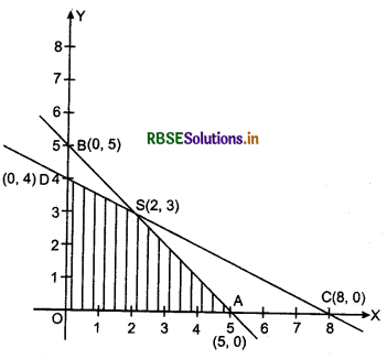
x + y = 5 ⇒ \(\frac{x}{5}+\frac{y}{5}\) = 1 which is clearly a straight line AB passing through points A (5, 0) and B(0,5).
Similarly, x + 2y = 8 ⇒ \(\frac{x}{8}+\frac{y}{4}\) = 1 which is clearly a line CD passing through points C(8,0) and D(0,4).
Constraints x ≥ 0 and y ≥ 0 represent only the required non-negative solution.

Third step (Feasible region):
Coordinates of 0(0, 0) satisfy both the inequalities x + y < 5 and x + 2y < 8. Hence, the shaded region lies on the side of the lines AB and CD containing 0(0, 0). In this way, shaded region OASDO is the feasible region which is clearly a convex polygon whose vertices are 0(0, 0), A (5, 0), S(2, 3) and D (0,4). Here, the values of x and y for P are obtained by solving equations x + y - 5 and x + 2y = 8 respectively.

Fourth step (Position of required point) :
Optimal value of the required point or objective function lies on any vertex of this convex polygon OASDO,

Fifth step (To find the required value of objective function):
We evaluate objective function P = 2x - y at each vertex of convex polygon OASDO :
A + O(0, 0), P = 2(0) - (0) = 0
A + A( 5,0), P = 2 × 5 - 0 = 10
A + S(2,3), P = 2 × 2 - 3 = 1
and D(0,4), P = 2 × 0 - 4 = -4
Thus, it is clear that the required minimum value of objective function P is - 4 at D(0,4).

(i) Feasible (optimal) Region and Solution : The common region determined by all the constraints including non-negative constraints x ≥ 0, y ≥ 0 of a LPP is called the feasible region for the LPP.
 Points within and on the boundary of the feasible region are called feasible solutions of the constraints. For example D(0, 4), S(2, 3) and A(5, 0) are the feasible solutions.
 
(ii) Optimal (Feasible) solution : any point in the feasible region that gives the optimal value (maximum or minimum) or the objective function is called on optimal solution.

Theorem 1.
Let R be the feasible region (convex polygon) for a linear programming problem and let Z = ax + by be the objective function. When Z has an optimal value (maximum or minimum), where the variables x and y are subject to the constraints described by linear inequalities, this optimal value must occur at a comer point (vertex) of the feasbile region.

Note: A comer point of a feasible region is a point in the region which is the intersection of two boundary lines.

Theorem 2.
Let R be the feasible region for a linear
programming problem and let Σ = ax + by be the objective function. If R is bounded, then the objective function Z has both a maximum and a minimum value of R and each of these occurs at a comer point (vertex) of R.   

Note : A feasible region of a system of linear inequalities is said to be bounded if it can be enclosed within a circle. Otherwise, it is called unbounded. Unbounded means that the feasible region does extend indefinitely in any direction.

Different Types of Linear Programming Problems:
A few improtant linear programming problems are listed below:

• Manufacturing Problems : In these problems, we determine the number of units of different products which should be produced and sold by a firm when each product requires a fixed manpower, machine hours, labour hour per unit of product, warehouse space per unit of the output etc, in order to make maximum profit.
• Diet Problems: In these problems, we determine the amount of different kinds of constituents/nutrients which should be included in a diet so as to minimise the cost of the desired diet such that it contains a certain minimum amount of each constituent/ nutrients.
• Transportation Problems : In these problems, we determine a transportation schedule in order to find the cheapest way of transporting a product from plants/factories situated at different locations to different markets. 

→    A linear programming problem is one that is concerned with finding the optimal value (maximum or minimum) of a linear function of serveral variables (called objective function) subject to the conditions that the variables are non-negative and satisfy a set of linear inequalities (called linear constraints). Variables are sometimes called decision variables and are non-negative.

→ A few important linear programming problems are :

• Diet problems
• Manufacturing problems
• Transportation problems.

→ The common region determined by all the constraints including the non-negative constraints x>0, y >0 of a linear programming problem is called the feasible region (or solution region) for the problem.

→ Points within and on the boundary of the feasible region represent feasible solutions of the constraints.
Any point outside the feasible region is an infeasible solution.

→ Any point in the feasible region that gives the optimal value (maximum or minimum) of the objective function is called an optimal solution.

→ The following Theorems are fundamental in solving linear programming problems:
Theorem 1.
Let R be the feasible region (convex polygon) for a linear programming problem and let Z = ax + by be the objective function. When Z has an optimal value (maximum and minimum), where the variables x and y are subject to constraints described by linear inequalities, this optimal value must occur at a corner point (vertex) of the feasible region.
 
Theorem 2 Let R be the feasible region for a linear pro¬gramming problem and let Z = ax + by be the objective function. If R is bounded, then the objective function Z has both a maximum and a minimum value of R and each of these occurs at a comer point (vertex) of R.

→ If the feasible region is unbounded, then a maximum or a minimum may not exist. However, if it exist, it must occurs at a comer point of R.

→ Comer point method for solving a linear programming problem. The method comprises of the following steps:

• Find the feasible region of the linear programming problem and determine its corner points (vertices).
• Evaluate the objective function Z = ax + by at each corner point. Let M and m respectively be the largest and smallest values at these points.
• If the feasible region is bounded, M and m respectively are the maximum and minimum values of the objective function.

If the feasible region is unbounded, then
(a) M is the maximum value of the objective function, if the open half plane determind by ax + by > M has no point in common with the feasible region. Otherwise, the objective function has no maximum value.
(b) m is the minimum value of the objective function, if the open half plane determined by ax + by < m has no point in common with the feasible region. Otherwise, the objective function has no minimum value.

→ If two corner points of the feasible region are both optimal solutions of the same type, i.e., both produce the same maximum or minimum, then any point on the line segment joining these two points is also an optimal solution of the same type.